We can go a long way in Machine Learning without having to deal with the scary probabilistic expressions. But, in order to be able to read the bleeding edge research as soon as it is published, and not from a blog, months later, we need to able to speak the language of probability. Probability is a great way to express the relationship between the data and the model, concisely. We are familiar with how Linear Regression works from Andrew Ng’s course. We know the loss function just tries to minimize the quadratic distance between data points and the model (line). In this post, we will revisit Linear Regression from a probabilistic perspective, using a method known as the Maximum Likelihood estimation. We could apply this knowledge to any Neural Network based architecture.
The principle of Maximum Likelihood is at the heart of Machine Learning. It guides us to find the best model in a search space of all models. In simple terms, Maximum Likelihood Estimation or MLE lets us choose a model (parameters) that explains the data (training set) better than all other models. For any given neural network architecture, the objective function can be derived based on the principle of Maximum Likelihood.
MLE is a tool based on probability. There are a few concepts in probability, that should be understood before diving into MLE. Probability is a framework for meauring and managing uncertainty. In machine learning, every inference we make, has some degree of uncertainty associated with it. It is essential for us to quantify this uncertainty. Let us start with the Gaussian Distribution.
Gaussian Distribution
A probability distribution is a function that provides us the probabilities of all possible outcomes of a stochastic process. It can be thought of, as a description of the stochastic process, in terms of the probabilities of events. The most commonly occurring distribution is the Gaussian Distribution or the Normal Distribution.
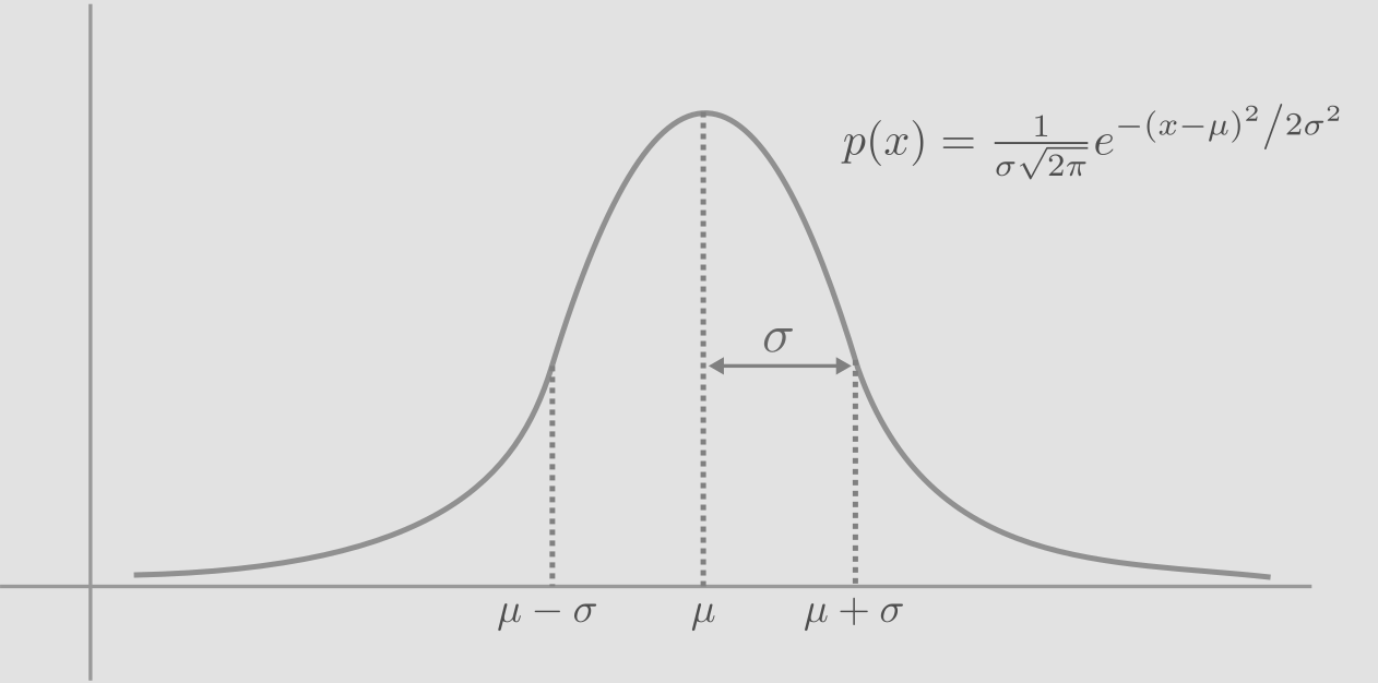
The gaussian distribution is a means to measure the uncertainty of a variable that is continuous between \(-\infty\) and \(+\infty\). The distribution is centered at mean, \(\mu\). The width depends on the parameter \(\sigma\), the standard deviation (variance, \(\sigma^{2}\)). Naturally, area under the curve equals 1.
Let us take the example of coin toss, to understand the normal distribution. We take an unbiased coin and flip it ‘n’ times. We calculate the probability of occurance of 1 to ‘n’ heads for each ‘n’ value. In the animation below, each frame is an experiment and the number on right top corner denotes the number of flips in that experiment. Each experiment involves flipping the coin ‘n’ times. We observe the probability of getting 1, 2,…‘n’ heads for each experiment, and plot it.
As you can see, with increase in number of flips (experiments), the curve of probability distribution tends to assume the shape of a normal distribution, represented by the equation above. In each of the experiments, the peak probability happens at half the number of heads and the probability density tends to decay on both sides. This is basically due to the fact that, there are more possible ways for the results to be close to half heads and half tails, compared to number of heads dominating the number of tail or vice versa.
That was fun to watch but how is this relevant to linear regression or machine learning? The data points in the training set, do not accurately represent the original data generating distribution or process. Hence we consider the process stochastic and build our model to accomodate a certain level of uncertainty. Every data point can be considered a random variable sampled from the data generating distribution which we assume to be gaussian. By that logic, learning or training is basically recreating the original distribution, that generated the training data.
Random Sampling
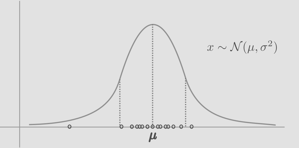
The process of sampling from a normal distribution is expressed as, \(x \sim \mathcal{N}(\mu, \sigma^{2})\). ‘x’ is a random variable sampled or generated or simulated from the guassian distribution. As we sample from this distribution, most samples will fall around the center, near the mean, because of higher probability density in the center.
Multivariate Gaussian
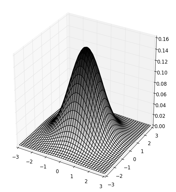
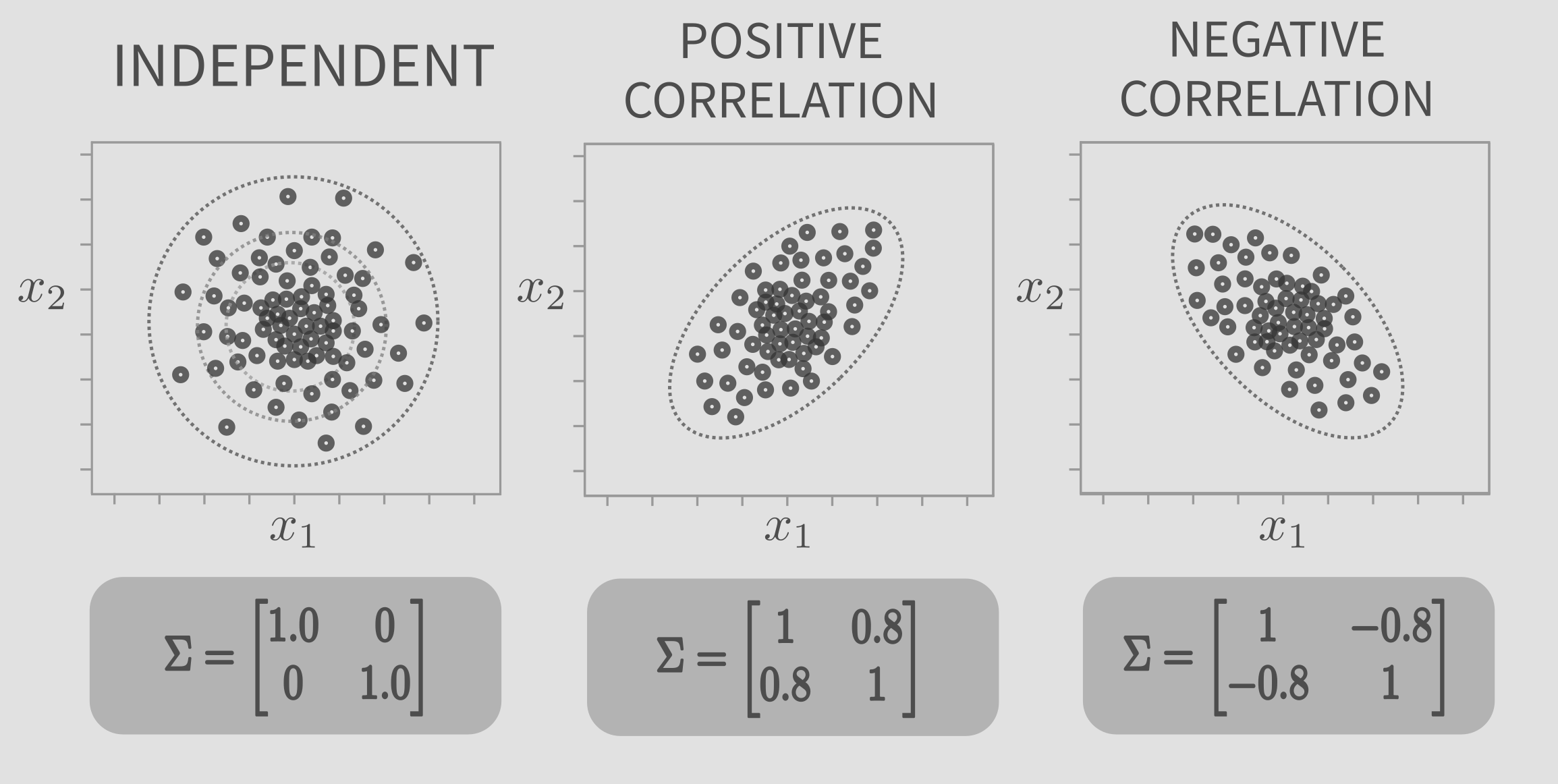
The 2D gaussian distribution or bivariate distribution, consists of 2 random variables \(x_1\) and \(x_2\). It can have many different shapes. The shape depends on the covariance matrix, \(\Sigma\). The Multivariate Gaussian Distribution is a generalization of bivariate distribution, for ‘n’ dimensions.
In the above expression, y and \(\mu\) are vectors of ‘n’ dimensions, and \(\Sigma\) is a matrix of shape ‘nxn’.
The figure below presents the top view of bivariate gaussian. The smaller circles denote the data points sampled from the distribution. Notice the variation in the shape of the gaussian with \(\Sigma\). The mean, given by \(x_1\) and \(x_2\) (\(\mu_1\) and \(\mu_2\)) determine the center of the gaussian, while \(\Sigma\) determines the shape.
Maximum Likelihood
I am borrowing this amazing toy example from Nando de Fretais’s lecture, to illustrate the principle of maximum likelihood. Consider 3 data points, \(y_1=1, y_2=0.5, y_3=1.5\), which are independent and drawn from a guassian with unknown mean \(\theta\) and variance 1. Let’s say we have two choices for \(\theta\) : {1, 2.5}. Which would you choose? Which model (\(\theta\)) would explain the data better?
In general, any data point drawn from a gaussian with mean \(\theta\) and and variance 1, can be written as,
\[y_i \sim \mathcal{N}(\theta, 1) = \theta + \mathcal{N}(0,1)\]\(\theta\), the mean, shifts the center of the standard normal distribution (\(\mu=0\) and \(\sigma^2=1\)).
The likelihood of data (\(y_1, y_2, y_3\)) having been drawn from \(\mathcal{N}(\theta,1)\), can be defined as,
\[P(y1,y2,y3 \vert \theta) = P(y1 \vert \theta) P(y2 \vert \theta) P(y3 \vert \theta)\]as \(y_1, y_2, y_3\) are independent.
Now, we have two normal distributions defined by \(\theta\) = 1 and \(\theta\) = 2.5. Let us draw both and plot the data points. In the figure below, notice the dotted lines that connect the bell curve to the data points. Consider the point \(y_2=0.5\) in the first distribution(\(\mathcal{N}(\mu=1, \sigma^2=1)\)). The length of the dotted line gives the probability of the \(y_2=0.5\) being drawn from \(\mathcal{N}(\mu=1, \sigma^2=1)\).
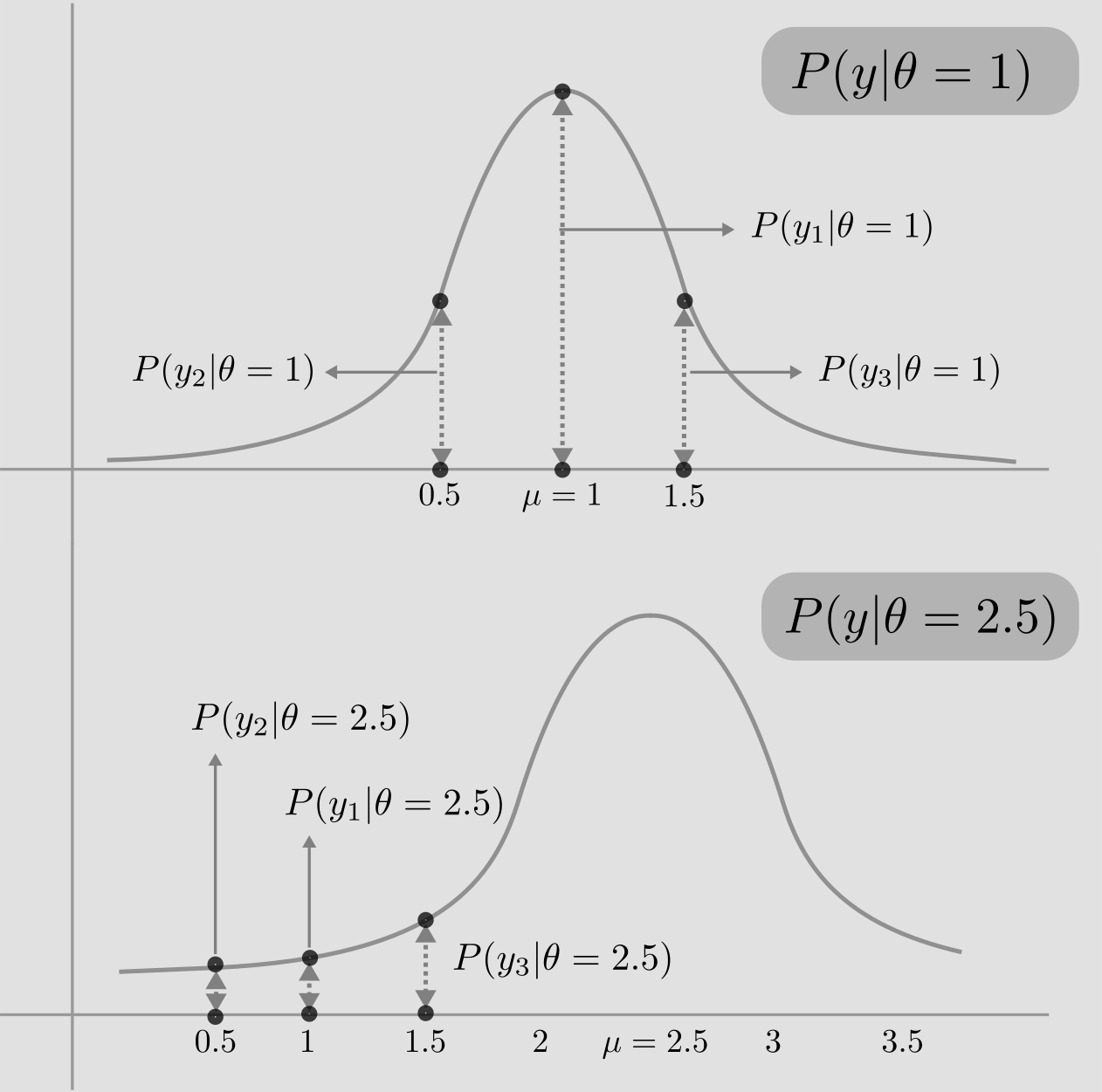
The likelihood of data (\(y_1, y_2, y_3\)) having been drawn from \(\mathcal{N}(\mu=1,\sigma^2=1)\), is given by,
\[P(y1,y2,y3 \vert \theta=1) = P(y1 \vert \theta=1) P(y2 \vert \theta=1) P(y3 \vert \theta=1)\]The individual probabilities in the equation above, are equal to the heights of corresponding dotted lines in the figure. We see that the likelihood, given by the product of individual probabilities of data points given model, is basically the product of lengths of dotted lines. It is obvious that the likelihood of model \(\theta = 1\) is higher. We choose the model (\(\theta = 1\)), that maximizes the likelihood.
Linear Regression
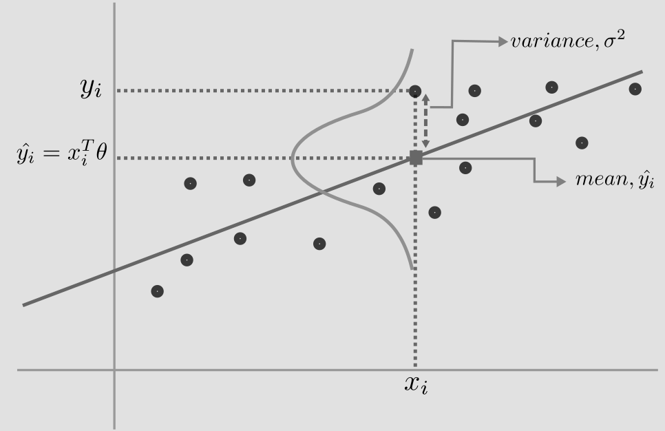
We are ready to apply MLE to linear regression, where the objective is to find the best line that fits the data points. But first, let us make some assumptions. We assume each label, \(y_i\), is gaussian distributed with mean, \(x_i^T\theta\) and variance, \(\sigma^2\), given by
\[y_i = \mathcal{N}(x_i^{T}\theta, \sigma^{2}) = x_i^{T}\theta + \mathcal{N}(0, \sigma^{2})\\ prediction, \hat{y_i} = x_i^T\theta\\\]where each \(x_i\) is a vector of form (\(x_i^1=1, x_i^2\)).
The mean, \(x_i^{T}\theta\) represents the best fit line. The data points will vary about the line, and the second term, captures this variance, \(\mathcal{N}(0, \sigma^{2})\) (see figure below).
Learning
If we assume that each point \(y_i\) is gaussian distributed, the process of learning becomes the process of maximizing the product of the individual probabilities, which is equivalent to maximizing the log likelihood. We switch to log space, as it is more convenient and it removes the exponential in the gaussian distribution.
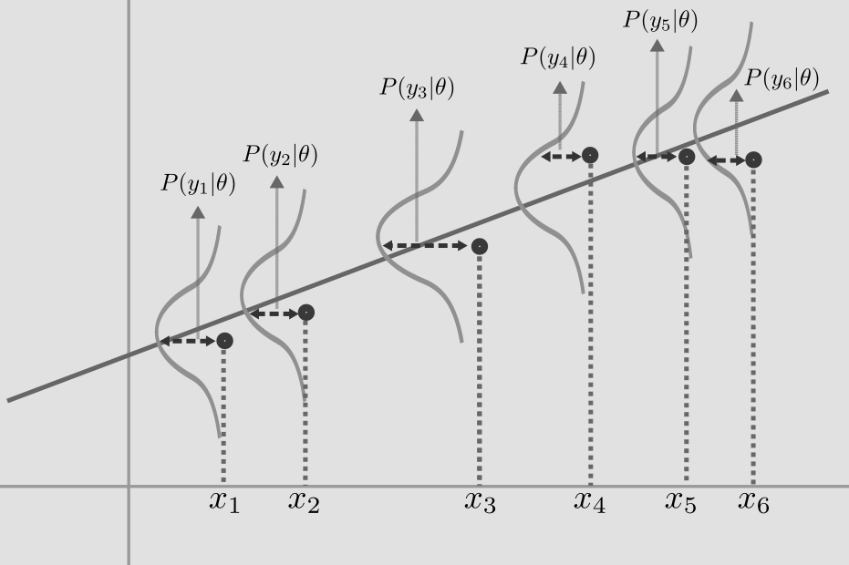
As the data points are independent, we can write the joint probability distribution of \(y, \theta, \sigma\) as,
\[p(y \vert X, \theta, \sigma) = \prod_{i=1}^{n} p(y_i \vert x_i, \theta, \sigma)\\ p(y \vert X, \theta, \sigma) = \prod_{i=1}^{n} (2\pi\sigma^2)^{-1/2} e^{-\frac{1}{2\sigma^2}(y_i - x_i^T\theta)^2}\]rewriting in vector form,
\[p(y \vert X, \theta, \sigma) = (2\pi\sigma^2)^{-n/2} e^{-\frac{1}{2\sigma^2}(y - X\theta)^T(y - X\theta)}\]Log likelihood,
\[l(\theta) = -\frac{n}{2}log(2\pi\sigma^2) -\frac{1}{2\sigma^2}(Y-X\theta)^T(Y-X\theta)\]The first term is a constant and the second term is a parabola, the peak (maxima) of which can be found by equating the derivative of \(l(\theta)\) to zero. Equating first derivative to zero, we get,
\[\frac{dl(\theta)}{d\theta} = 0 = -\frac{1}{2\sigma^2}(0 - 2X^TY + X^TX\theta)\]we get,
\[\hat{\theta_{ML}} = (X^TX)^{-1}X^TY\]Finally, we reach our goal of finding the best model for linear regression. This equation is commonly known as the normal equation. The same equation can be derived using the least squares method (perhaps in another post).
Similarly, we can get the maximum likelihood of variance, \(\sigma^2\), by differentiating log likelihood with respect to \(\sigma\) and equating to zero.
\[\hat{\sigma}^2_{ML} = \frac{1}{n} (Y-X\theta)^T(Y-X\theta) = \frac{1}{n}\sum_{i=1}{n}(y_i - x_i\theta)^2\]This gives us the standard estimate of variance in the training data.
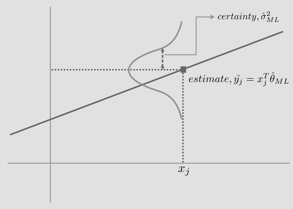
Inference
So, we have learned the parameters of our model, \(\hat{\theta}_{ML}\) and \(\hat{\sigma}^2_{ML}\). Based on these learned parameters, we can make inferences for new unseen data. For a new data point \(x_j\), our best estimate is given by,
\[estimate, \hat{y_j} = x_j^T\hat{\theta}_{ML}\]The degree of uncertainty in our estimate, is given by the variance, \(\hat{\sigma}^2_{ML}\).
Reference
- Andrew Ng’s Machine Learning course
- Nando de Freitas’s Machine Learning course
- Maximum Likelihood and Linear Regression
- Coin Toss Experiment
- Bivariate Gaussian in matplotlib
I hope to do a follow up post very soon, applying maximum likelihood to more complex neural networks, and also introduce the concept of Bayesian Learning and compare it with the Frequentist approach.
Feel free to drop a comment.